Basics examples
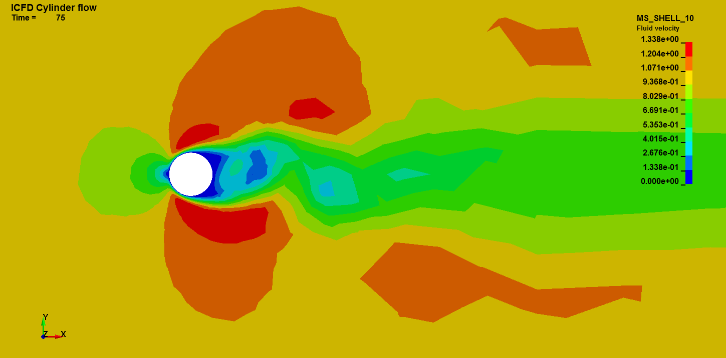
Basics : Cylinder flow
This LS-DYNA simulation shows a simple ICFD input deck with a coarse mesh. The inflow is characterized by a prescribed velocity while the reference pressure has been set to 0 for the outlet (undisturbed flow). For the far field domain, a freeslip boundary condition has been used, stipulating that the normal component of the velocity is null while the tangential is left free. For those conditions to be physically valid, they need to be put far away for the object of interest in this case the cylinder. The volume mesh is generated automatically and a boundary layer mesh has been applied to the cylinder in order to better capture the velocity gradient close to the wall.
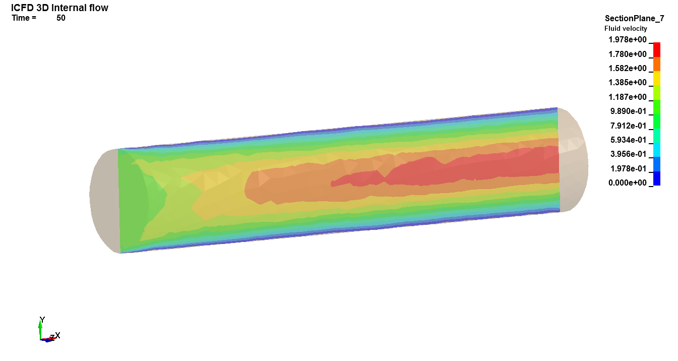
Basics : Internal 3D flow
This LS-DYNA simulation shows a simple 3D ICFD problem. It features a flow through a cylindrical pipe. Since the Reynolds number is laminar, a parabolic profile is expected at the outlet. It makes use of the ICFD_CONTROL_SURFMESH keyword to remesh the original surface mesh. The purpose of the ICFD_CONTROL_MESH in this input deck is to add more elements through the cylinder's diameter. It is also a good example for the MESH_BL_SYM keyword. The user can comment that keyword to see its impact on the mesh close to the inlet or outlet.
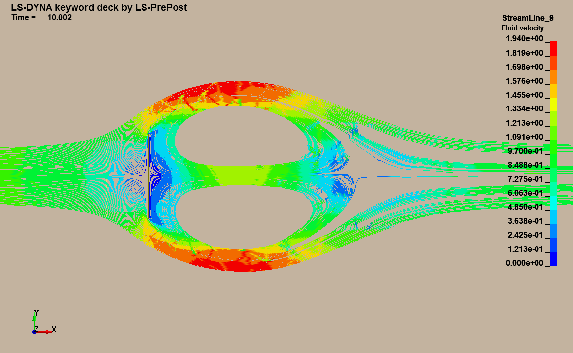
Basics : Plate flow
This LS-DYNA simulation shows a simple ICFD input deck with a coarse mesh. It shows how the solver deal with infinitely thin plates or shells in 3D. Since two nodes are needed in order to solve for the pressure difference between the two faces of the plate, the automatic volume mesher will generate an extra node and 'pull' a little on the mesh leaving a tiny gap between them, considered infinitely small compared to the size of the problem. This is done through the introduction of the keyword MESH_EMBEDSHELL.
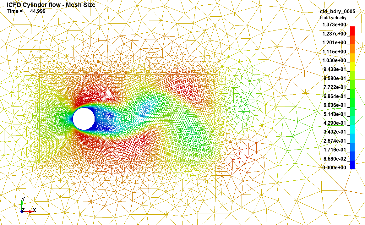
Basics : Mesh Size
This LS-DYNA simulation is a simple modification of the flow around the cylinder example. Another part is created within the fluid volume. The nodes of this part are then added to the volume mesh using MESH_SIZE. This method is the most robust way to define zones within the mesh that need to maintain a finer element size. Alternatively, a quick method to define a specific shape where a certain element size has to be maintained is through the use of the MESH_SIZE_SHAPE keyword. The user is encouraged to try both methods and to observe the differences between the two meshes generated.
Basics : Thermal flow
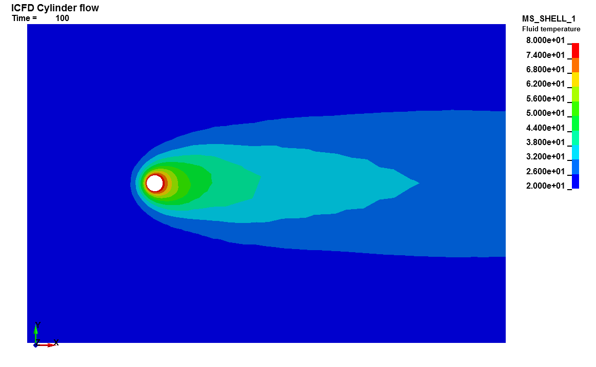
This LS-DYNA simulation shows a simple ICFD forced convection input deck with a coarse mesh. Compared to the basic cylinder flow problem, this problem adds the keywords to solve the heat equation. A 20 degree cooling wave flows over a hot cylinder that maintains a constant temperature of 80 degrees. The domain is initialized at 10 degrees.
Basics : Free Convection flow
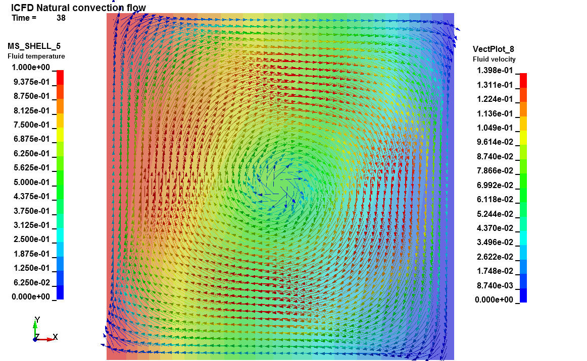
This LS-DYNA simulation shows a simple ICFD free convection problem. Since the solver is incompressible, density is a constant. Instead, the tiny density variations due to the rise in temperature are approximated by a external force applied on the system and function of the fluid's thermal expansion coefficient, gravity and fluid temperature (Boussinesq approximation). Depending on the Raleigh number value, different vortex behaviors can be observed.

Basics : User defined mesh
This LS-DYNA simulation shows a simple flow around a cylinder case. However, instead of being generated automatically, the volume mesh is provided as input by the user. The user is encouraged to compare this example to the Basics : Cylinder flow example to see what keywords needed to be modified, added or removed.
Basics : Dam break
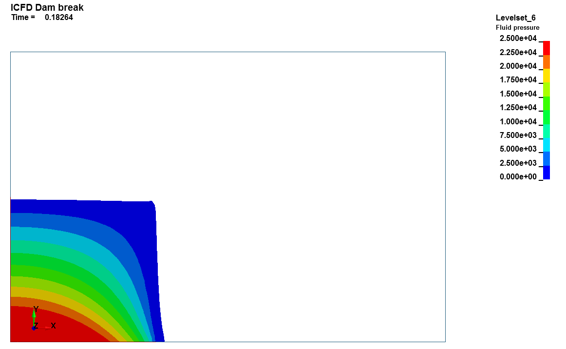
This LS-DYNA simulation shows a simple free surface example using the ICFD solver. A column of water collapses under the load of gravity. In order to set up such a problem, the domain must be divided in two ICFD_PART_VOLs, one for the fluid, one for the vacuum. For the automatic volume mesher to recognize the initial interface, the keyword MESH_INTERF must be used. Gravity load is applied through the use of LOAD_BODY keyword. Since the solver is implicit, no ramp up is needed.
Basics : Wave Generation
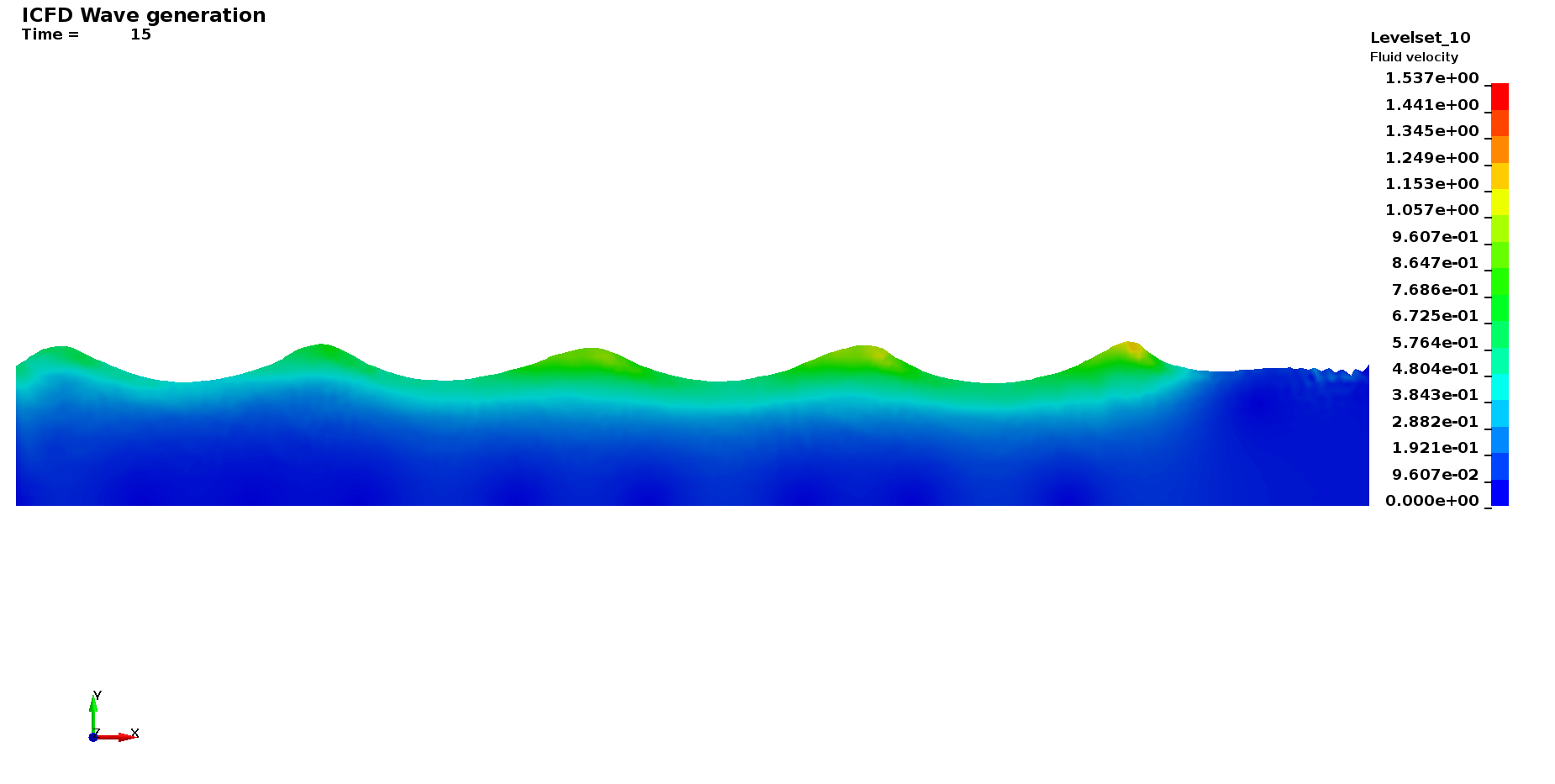
This LS-DYNA simulation shows how to set up a simple wave generation problem using Stokes waves. This wave modelling is suitable in cases where the wave amplitude is small compared to the total depth of the problem. Otherwise, piston-type waves are preferred. A hydrostatic pressure condition has been set at the outlet in order to allow for some fluid to leave the domain. In addition, a damping layer close to the outlet has been defined in order to increase the problem's stability and to avoid reflection of the waves.
Basics : Driven Cavity
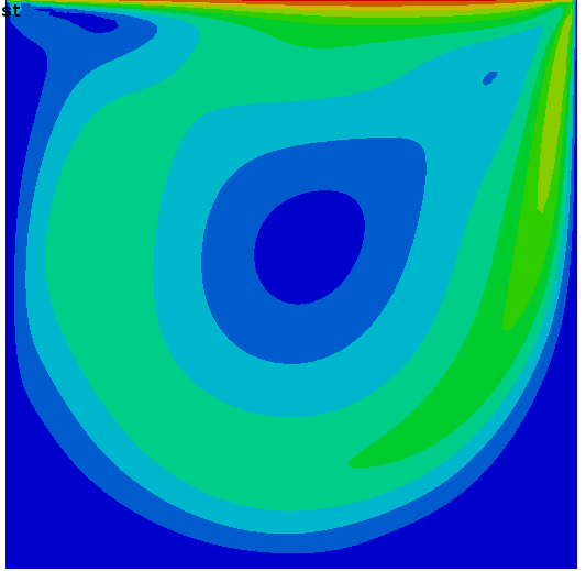
This is the universally famous driven cavity case tested with the second order steady solver and for Re=1000.

Basics : Backward facing step
The 2D laminar backward facing step is a widely encountered benchmark for CFD code testing. The present example features a mesh size of 0.05 and a Reynolds number of 800. The second order steady state solver is used, requires LS-DYNA MPP Dev 114223 (or higher) with double precision.
Basics : Weak FSI
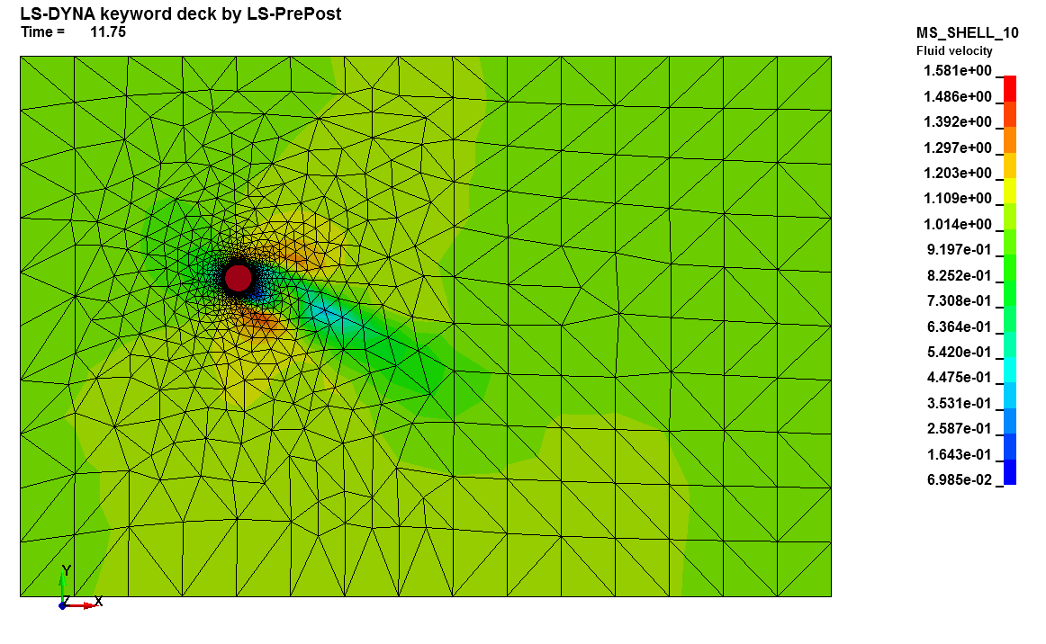
This LS-DYNA simulation shows a simple FSI coupling problem using weak/loose/explicit FSI. A rigid cylinder has a prescribed displacement in the Y direction. After five seconds, the inlet velocity boundary condition is triggered pushing the cylinder to the right. Since the coupling is loose, the two solvers retain their own independent timesteps and the solid mechanics solver runs in explicit. The FSI uses a boundary fitted approach. The fluid mesh must have a boundary with the structure. The meshes do not have to coincide but the geometries must remain close. When FSI is triggered, the fluid mesh moves in a Lagrangian way while the fluid flow evolves in a Eulerian way.
Basics : Strong FSI
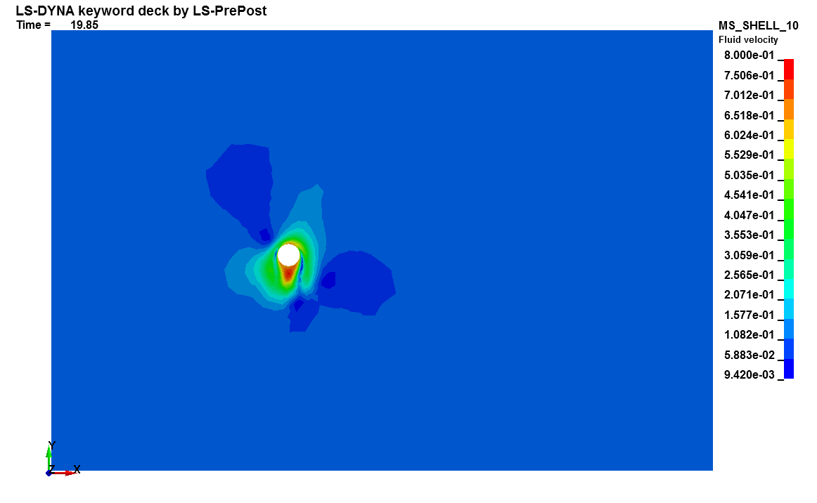
This LS-DYNA simulation shows a simple FSI coupling problem using strong FSI. Indeed, the density of the solid and the fluid are very close. Such cases are by definition unstable when using explicit coupling between solid mechanics and a CFD code ('added mass effect'). In order to reduce those instabilities, strong fluid structure interaction is needed. In order for this to be possible, both solvers need to advance at the same time thus making the use of the implicit solver for solids mandatory.
Basics : Imposed Move
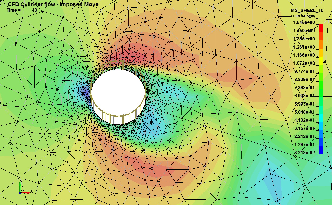
When doing FSI, it is possible through the keyword ICFD_CONTROL_FSI to trigger one way coupling i.e either only the fluid has an influence on the solid's displacements or only the solid has an influence on the fluid's flow pattern. The latter case is often used. However, this implies setting up the solid problem, solving it and communicating the solid's displacement and velocity to the fluid solver during the run which the fluid solver will then use to up move the volume mesh. In order to reduce calculation time and increase accuracy, it is often wise to directly impose the displacements on the fluid nodes through the use of the ICFD_CONTROL_IMPOSED_MOVE keyword.
Basics : Mesh Adaptivity
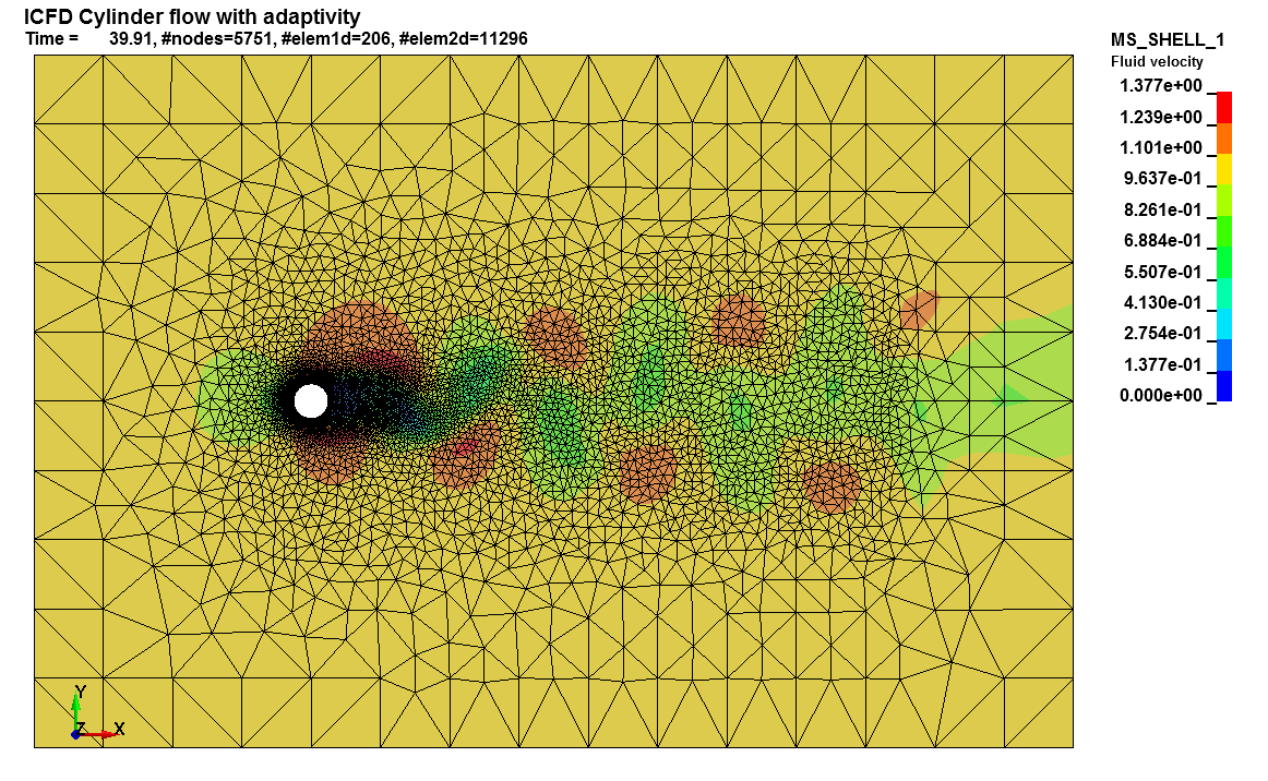
This LS-DYNA simulation shows a simple FSI coupling problem using weak/loose/explicit FSI. A rigid cylinder has a prescribed displacement in the Y direction. After five seconds, the inlet velocity boundary condition is triggered pushing the cylinder to the right. Since the coupling is loose, the two solvers retain their own independent timesteps and the solid mechanics solver runs in explicit. The FSI uses a boundary fitted approach. The fluid mesh must have a boundary with the structure. The meshes do not have to coincide but the geometries must remain close. When FSI is triggered, the fluid mesh moves in a Lagrangian way while the fluid flow evolves in a Eulerian way.
Basics : Mesh Morphing
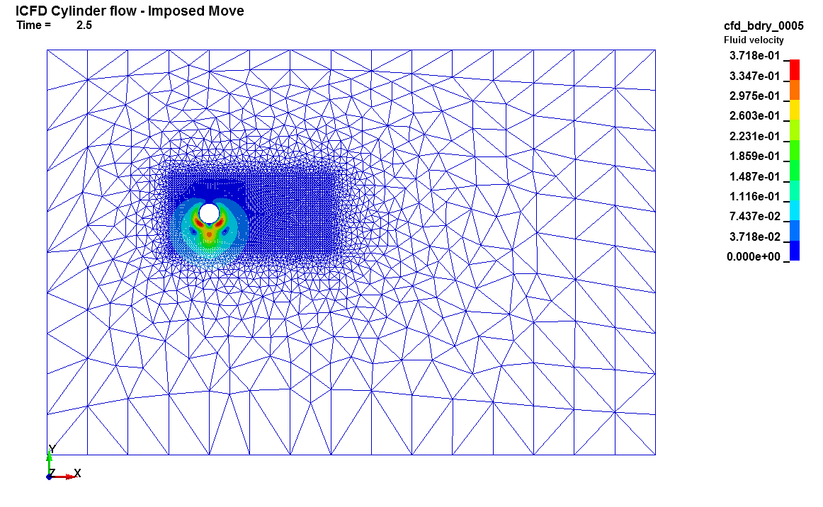
In some cases with imposed Lagrangian displacements, it may be interesting to keep the node topology close to the object of interest. This can save calculation time and may increase accuracy. This can be done by defining two separate volumes and by imposing the displacement on a volume through the use of ICFD_CONTROL_IMPOSED_MOVE. The interface between the two volumes is then defined by MESH_INTERF. This is not compatible with remeshing.
Basics : Conjugate heat transfer
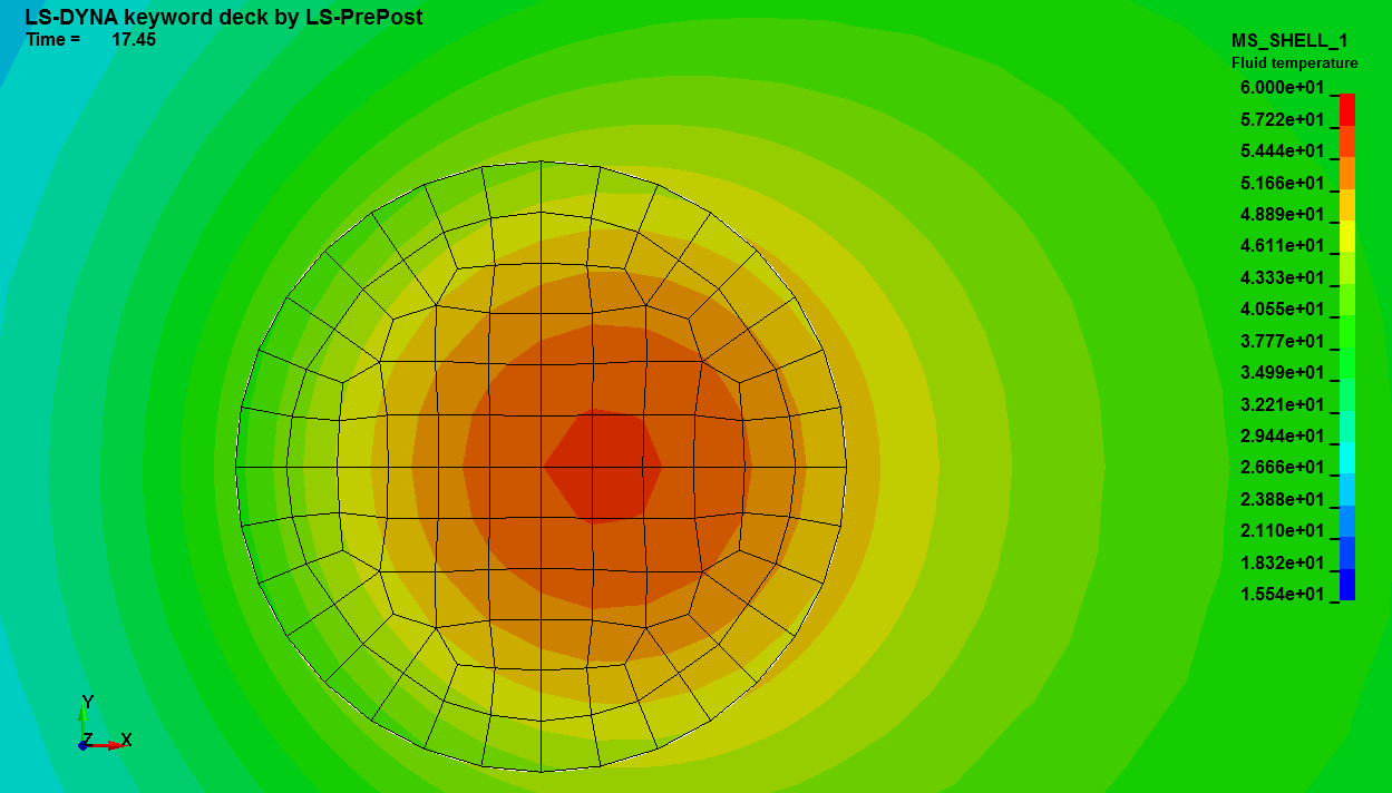
This LS-DYNA simulation shows a simple conjugate heat transfer problem. The default coupling method between the structure and the fluid is a robust monolithic strong coupling approach which allows for accurate solutions. In order to trigger the conjugate heat transfer solver, the FSI keywords must be defined as well, since the FSI algorithm is needed in order to detect which nodes belong to the fluid/solid interface. Of course, the corresponding solid thermal input deck must be set up.
Basics : DEM coupling
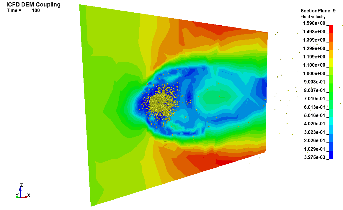
It is possible to couple the ICFD fluid solver with DEM particles. This feature can useful in cases involving mud, dust or snow deposition. The coupling is explicit and based on the particle drag coefficient and force.
Basics : Non Newtonian fluid
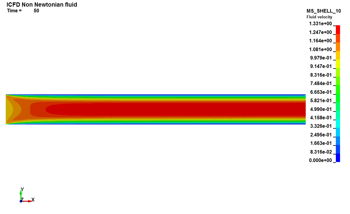
This ICFD input deck is a simple example featuring a Non-Newtonian fluid flowing through a 2D pipe. The model chosen is a Power Law. The user is encouraged to check the velocity profile at the outlet and to compare it to the classic Poiseuille parabolic profile.
Basics : Porous Media flow
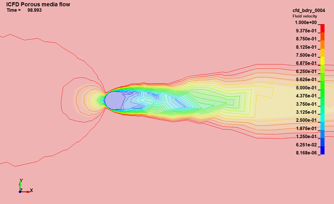
This LS-DYNA simulation shows a simple ICFD isotropic porous media flow input deck. Compared to the original cylinder flow, the cylinder now represents a porous media through which flow is allowed to flow albeit slowly. Several porous media models are available, the one used in this example is the Ergun correlation.
Basics : Anisotropic Porous Media flow
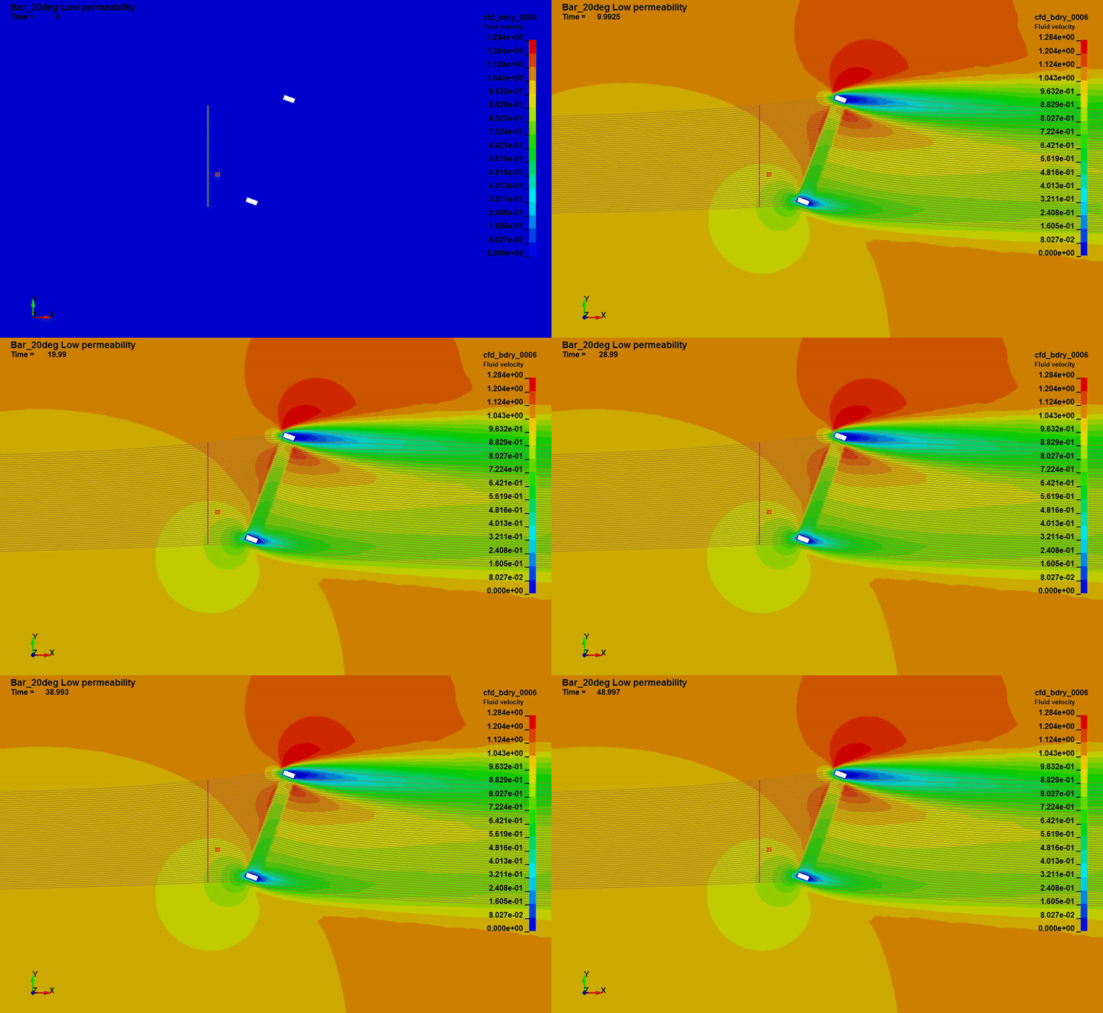
This LS-DYNA simulation shows a simple ICFD anisotropic porous media flow input deck. The flow entering the porous media is deflected and follows the orientation of the porous media.
Basics : Cylinder flow FSI
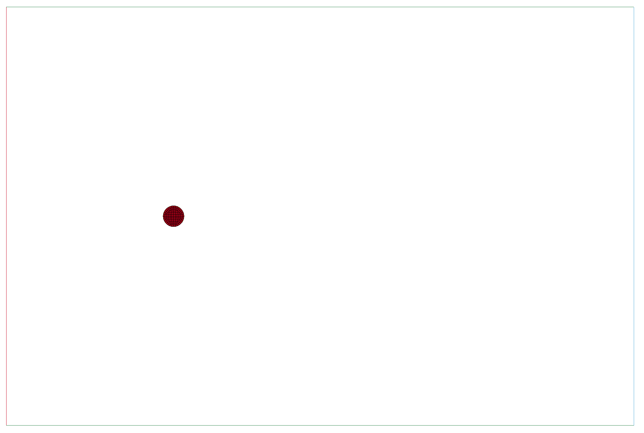
This LS-DYNA simulation is a extension to the Basics : Cylinder flow where a structural part is added and the FSI problem is solved. The structural part is fixed in all direction except the vertical direction, the fluid deck is the same and the only modification is the time step to save computational time.
Basics : Free liquid sloshing
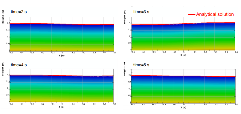
This validation sloshing simulation compares the free surface height to an analytical reference result.
Basics : Piston wave maker
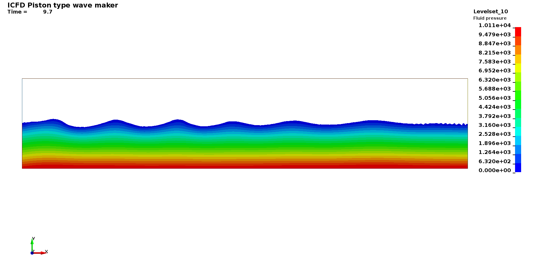
Piston wavemakers are used where the water is shallow compared to the wavelength of the waves. It is possible to generate such waves by imposing a periodic Lagrangian movement to one end of the domain. The waves are then damped on the other side.
Basics : Rotating reference frame II
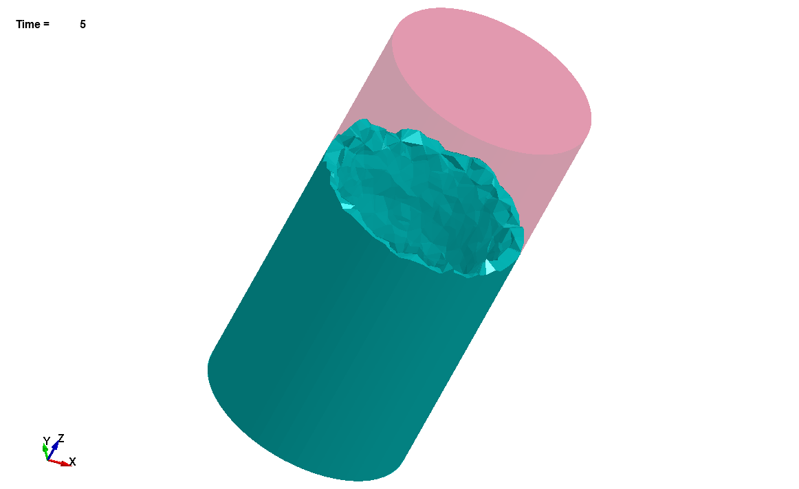
The free surface of a spinning half filled tank adopts a parabolic profile following an analytical law. This examples highlights this behavior by using the non inertial reference frame feature.
Basics : Rugosity flow
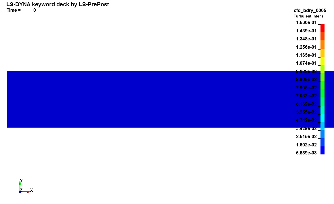
This LS-DYNA simulation shows an atmospheric air flow going over a rough surface. The Standard k-epsilon model is activated through the use of ICFD_CONTROL_TURBULENCE. Furthermore, the rugosity parameters have been defined. The user is invited to change those parameters and check the influence on the surface shear vector. The mesh size has been chosen so that a Y+ of approximately 30 is maintained over the domain.
Basics : Sloshing
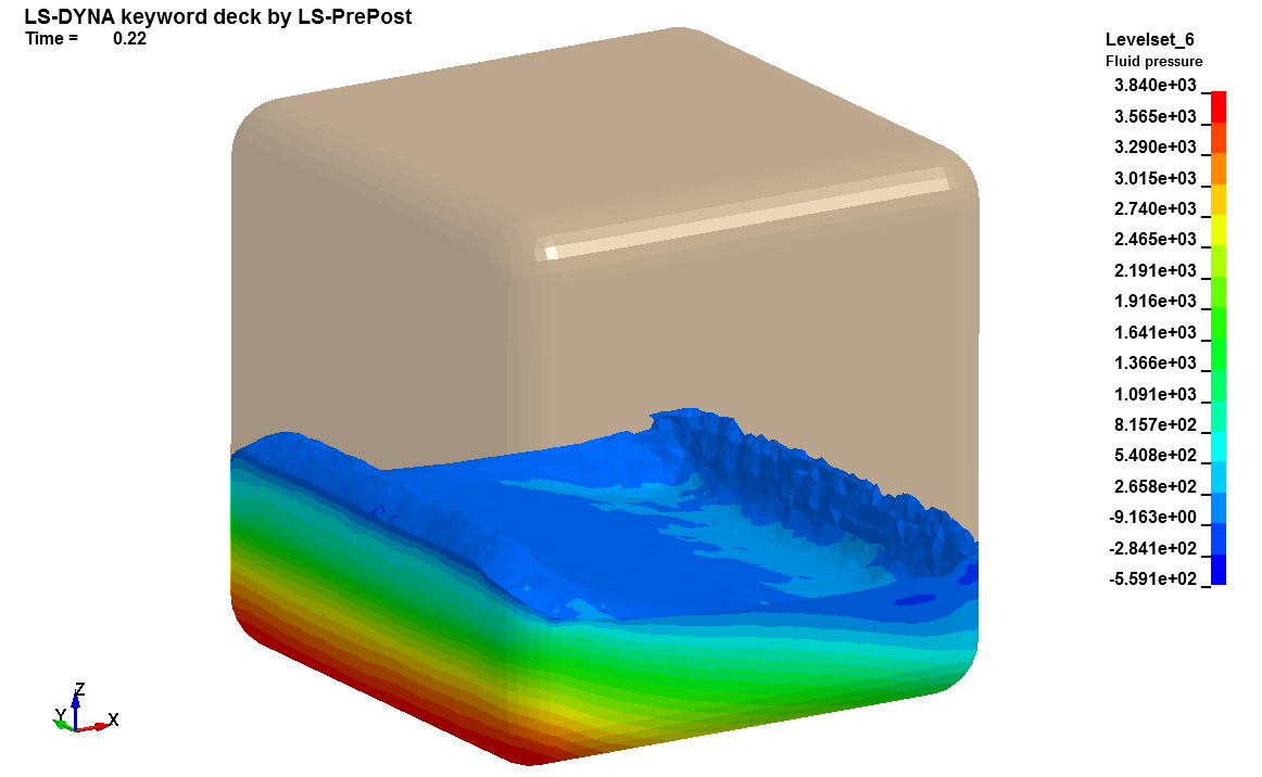
It is possible to directly impose a displacement of the entire volume mesh through the use of the keyword ICFD_CONTROL_IMPOSED_MOVE. This configuration can been encountered in sloshing type applications. The current input deck is a simple example of ICFD_CONTROL_IMPOSED_MOVE combined with a free surface configuration.
Basics : Turbulent flow
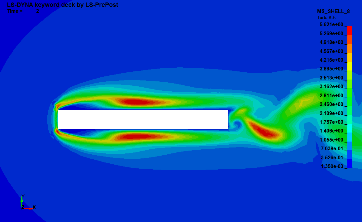
This LS-DYNA simulation shows a turbulent flow input deck. The fluid and boundary conditions give a Reynolds number of 50 000 making the flow turbulent and prompting the use of a turbulence model. The default configuration uses a RANS realizable model. The boundary layer mesh has been chosen in accordance, to yield an approximate Y+ value of 30. Several other turbulence models can be tried and the boundary layer mesh changed accordingly. The user can study the length and effects of the recirculation zone over the thick plate.
Basics : Weak thermal coupling
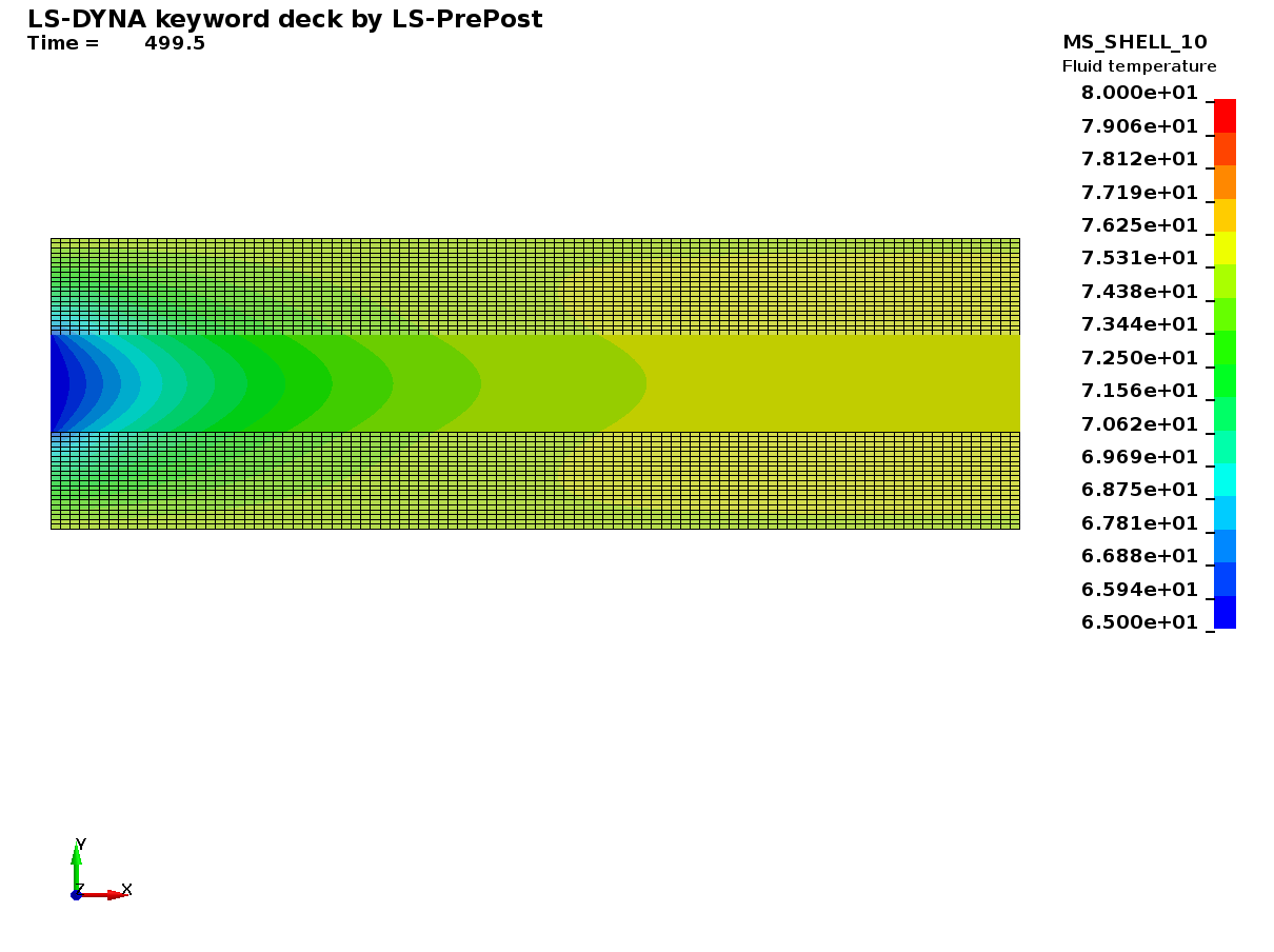
Besides the monolithic thermal coupling method, it is also possible to trigger a weak/loose explicit method between the structure and the fluid. The choice between the two methods can be made using ICFD_CONTROL_CONJ. This method may offer an alternative for lower computational time but a finer mesh may be necessary to achieve the same level of accuracy especially in the wall region. Similarly, the thermal and fluid timesteps may be independent but it is recommended to keep them close in highly non linear configurations. Regardless of the chosen coupling method, it is also possible to extract the heat transfer coefficient at the interface using ICFD_DATABASE_HTC. The user is encouraged to switch between the two coupling methods and compare.
Basics : Potential flow
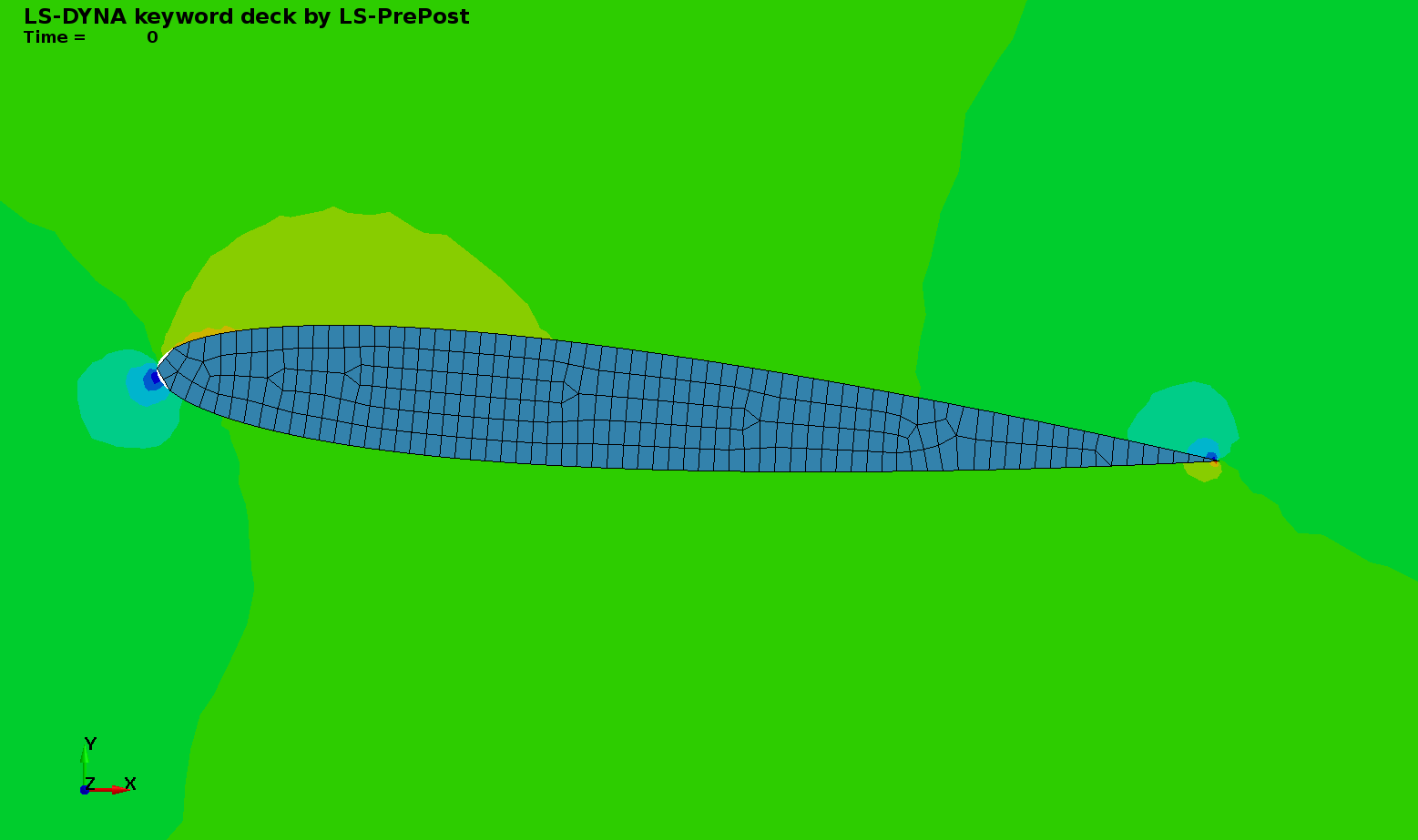
Despite its limitations (no boundary layer effects, irrotational flow), the solution given by a potential flow solver is very fast and can be used in certain configuration to give a quick approximation of the fluid flow. In this example, after the solve of the potential flow, the pressure is passed to the solid mechanics solver (linear FSI) and the vibrations of the structure can be analysed.
Basics : Rayleigh-Taylor
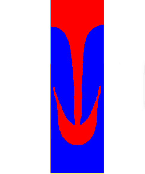
This example shows how to set up a simulation of two-phase flow with surface tension. Rayleigh-Taylor instability occurs when a fluid is on top of a lighter one.
Basics : Rising Bubble
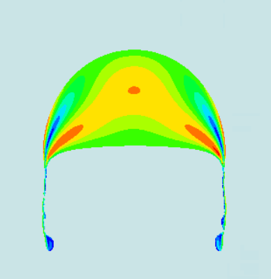
This input is based of the famous 2D rising bubble benchmark problem used to evaluate numerical algorithms for bi-phasic flow and surface tension. It uses some features of the levelset solver introduced in LS-DYNA R15. The levelset advection uses a semi Lagrangian approach. The levelset re-initialization uses a closest Point algorithm and the Laplace-Beltrami approach is used to handle the surface tension effects at the interface between the two fluids.
